Codenano, a tool for designing DNA nanostructures
Here, we give an introduction to what codenano can and can not do. The source code for codenano is hosted on a github repository: https://github.com/thenlevy/codenano, along with a short tutorial, and on crates.io. Update: 2020-10-31, although the source is aaiabile for people to use, codenano is no longer actively mainted by the group.
Designing DNA nanostructures using codenano
Codenano allows one to design and visualise DNA nanostructures specified using code, all in your browser. Codenano also has the ability to compute some simple interactions between DNA bases in order to help the user design DNA nanostructures that are feasible according to some simple criteria.
Creating nanostructures designs can be a tedious process and codenano is designed to make it less so. Codenano gives a simple API where one uses a small, simple, subset of the Rust programming language to specify a DNA nanostructure. Using this API does not require any knowledge of Rust. However, advanced users can benefit from the full expressiveness of Rust.

Codenano allows you to design DNA nanostructures in your web browser.
DNA nanostructures

Examples of DNA Origami structures presented in the original DNA origami article paper (Rothemund. Nature 440.7082 (2006): 297).
DNA nanostructures are small objects with nanoscale features typically made out of artificially synthesised DNA. For example, DNA Origami is a technique introduced by Paul Rothemund whereby a long strand of DNA called the scaffold is folded into a specified shape by using short (~32 DNA bases long) strands called staples. The staples bind to several distant regions of the scaffold and bring them close to each other. It is this biding of the staples to the scaffold that creates the shape. Other DNA nanostructures, such as the DNA tile lattices first designed by Ned Seeman, can be specified be designing a collection of short DNA strands that bind together.
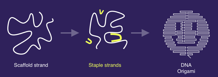 Principle of DNA origami, image by Aaron Berliner.
Existing tools
Several tools have been developed to provide assistance during the design process of DNA origami and other DNA nanostructures.
cadnano, is a widely used tool that cadnano offers a 2D drawing interface and a 3D visualisation of the structure being designed. However, cadnano designs cannot be easily edited programmatically, which would often be desirable. Moreover, its visualisation is limited to a 2D representation of secondary structures.
The VHelix plugin for Autodesk Maya, offers a 3D visualisation interface and allows the creation of wireframe designs, and other complex designs.
To gain insight into the physical feasibility of a design, a cadnano design can be given to CanDo, which runs a finite element-based simulation.
oxDNA is a simulation tool that includes thermodynamic and mechanical properties of DNA and RNA and has been used to model DNA nanostructures. Other software can be used for molecular simulation like MrDNA (multi-resolution simulations of self-assembled DNA nanostructures). Multistrand is a kinetic simulator of interacting DNA strands, typically useful for looking at DNA binding kinetics, such as toehold mediated strand displacement, but could be helpful for some aspects of nanostructure design. Finally, one can use molecular dynamic simulators when more fine-grained simulation is required, such as GROMACS.
How codenano can help you to design DNA nanostructures
There are two main ways to use codenano.
First, to script a design. When using codenano to specify a design, the structure is first drawn in the browser. We call this the unrelaxed design. This design is created by the user, using a rust API. See the tutorial.
Second, codenano can compute a "relaxed" form of the design, i.e. a configuration which is the result of attempting to satisfy a number of spring-based constraints described below. If the unrelaxed shape is not too different from the relaxed one the user may consider that unrelaxed shape is feasible according to our spring-based criteria.
Buyer beware! The codenano relaxation procedure uses a simplified model of DNA interactions that excludes many physical features that really do matter when designing good nanostructures.
Typically, the user might consider their design to have problems if according to codenano's relaxation:
- Some nucleotides in the relaxed shape are far from their intended position (to satisfy covalent and hydrogen bond lengths constraints, codenano is choosing to break stacks apart).
- Some helices intersect each other in the relaxed shape.
However, seeing these kinds of problems does not necessarily imply that the design will not work in the lab! Fixing the design might be as simple as rotating a few helices in the code that specifies the design -- something that the molecules would do by themselves in solution. Indeed, since codenano does not model many important DNA interactions, perhaps no fixing of the design is required at all.
As mentioned in the Future work section below, there are a number of properties of DNA excluded from codenano's relaxation procedure. Excluded features include steric hindrance (codenano allows helices to intersect each other); stacks that are not running along a perfect DNA duplex (hence a stack with a nick, or a pair of strand ends and all other kinds of loop and stacking interactions are excluded); and breaking of hydrogen bonds (e.g. due to strain or temperature; codenano will break/stretch stacks but not hydrogen bonds).
Examples
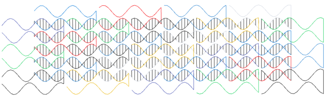
Example: Single-stranded tiles and choice of domain length
Here we use codenano to design a structure with single-stranded tiles similar to those of Wei, Dai and Yin in their paper Complex shapes self-assembled from single-stranded DNA tiles, Nature, 485(7400):623, 2012. Each tile is made of 4 short domains: 2 pairs of 2 domains where in each pair one domain is 10 bases long and the other domain is 11 bases long.
Single stranded tile design. Domains are of length 10 or 11 bases.
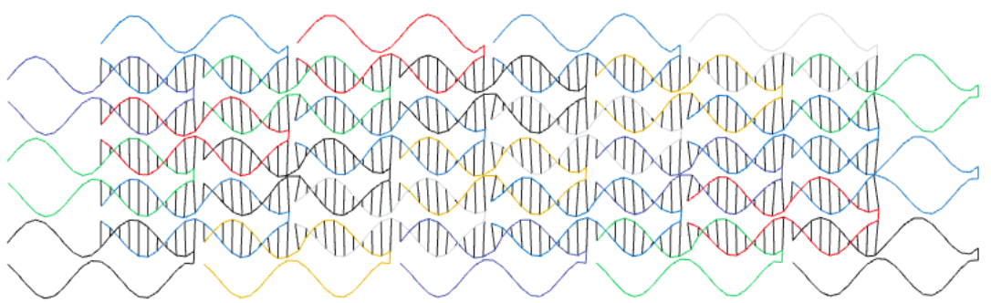
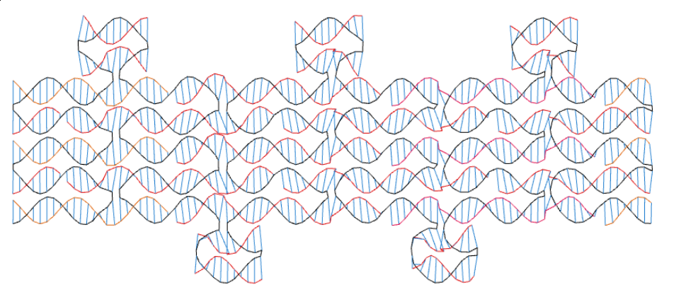
The relaxed form of the previous design, as computed by codenano.
Note that a small change to the design could make the design much worse, according to codenano. Here is what we get when all domains are 11 bases long:
Single-stranded tile design with all domains being of length 11 bases.
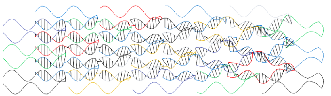
The relaxed form of the previous design.
Example: Large 2D lattice of single-stranded tiles
Since single-stranded tiles use a simple pattern that is repeated, we can design big large structures with a relatively short piece of code.
use codenano::*;
const half_tile_length:isize = 21;
pub fn add_sst(ori: &mut Nanostructure, helix_id: usize, helix_pos: isize,
len:isize) {
ori.draw_strand(helix_id, false, helix_pos, helix_pos + len - 1,
AUTO_COLOR);
ori.draw_strand(helix_id + 1, true, helix_pos + len - 1, helix_pos,
AUTO_COLOR);
ori.make_jump(ori.get_nucl(helix_id, helix_pos +len - 1, false),
ori.get_nucl(helix_id + 1, helix_pos + len - 1, true));
}
pub fn main() {
let mut ori = Nanostructure::new();
let id : Vec<usize> = (0..20).map(|i| ori.add_grid_helix(i, 0)).collect();
let mut shift = 6;
for i in 0isize..8 {
for j in 0usize..9 {
add_sst(&mut ori, j * 2, shift, half_tile_length);
add_sst(&mut ori, j * 2 + 1,
shift + half_tile_length/2, half_tile_length);
}
shift += half_tile_length;
}
let i = 8;
for j in 0usize..9 {
add_sst(&mut ori, j * 2, shift, half_tile_length);
}
ori.finish();
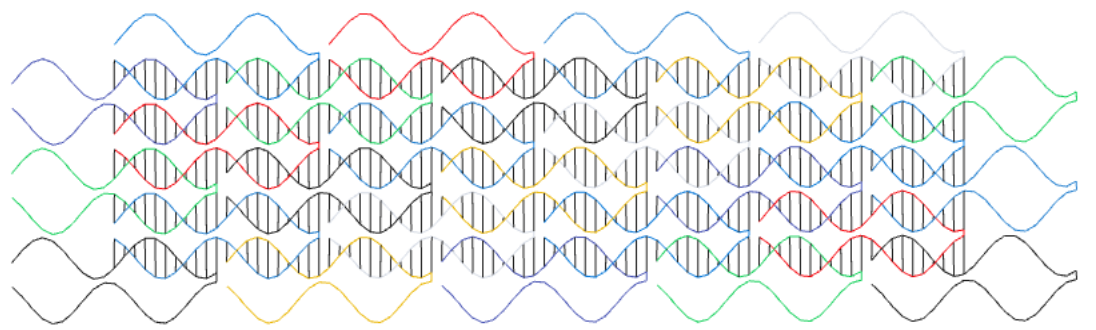
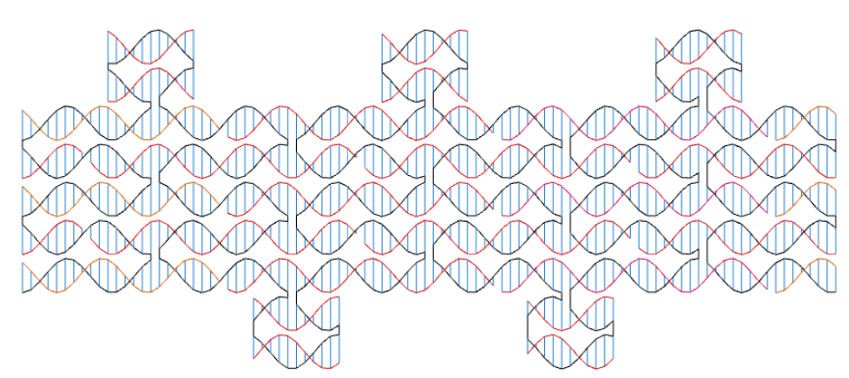
}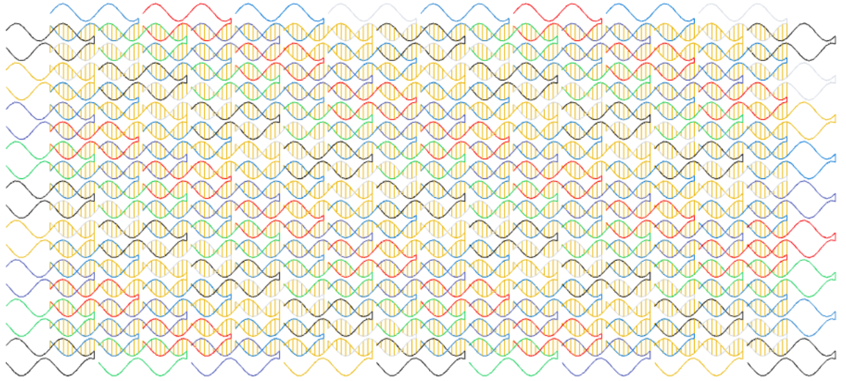 A large single-stranded tile structure designed with the above code.
Example: 3D shape
The previous code can be adapted a little bit to produce a 3D shape. To do that we create more helices and put them on different places of the grid. (In codenano, press Alt and move the mouse to rotate the view).
use codenano::*;

const half_tile_length:isize = 21;
pub fn add_sst(ori: &mut Nanostructure, helix_id: usize, helix_pos: isize,
               len:isize) {
        ori.draw_strand(helix_id, false, helix_pos, helix_pos + len - 1,
                        AUTO_COLOR);
        ori.draw_strand(helix_id + 1, true, helix_pos + len - 1, helix_pos,
                        AUTO_COLOR);
        ori.make_jump(ori.get_nucl(helix_id, helix_pos +len - 1, false),
                      ori.get_nucl(helix_id + 1, helix_pos + len - 1, true));
}

pub fn main() {

    let mut ori = Nanostructure::new();
    (0..10).map(|i| ori.add_grid_helix(i, i)).collect::<Vec<_>>();
    (0..10).map(|i| ori.add_grid_helix(10 + i, 9 - i)).collect::<Vec<_>>();
    (0..10).map(|i| ori.add_grid_helix(10 + (9 -i), -10 + (9 -i))).collect::<Vec<_>>();

    (0..10).map(|i| ori.add_grid_helix(9 - i ,  -(9 - i) - 1 )).collect::<Vec<_>>();
    let mut shift = 7;
    for i in 0isize..3 {
        for j in 0usize..19 {
            add_sst(&mut ori, j * 2, shift, half_tile_length);
            add_sst(&mut ori, j * 2 + 1,
                    shift + half_tile_length/2, half_tile_length);
        }

        shift += half_tile_length;

    }
    let i = 3;
    for j in 0usize..17 {
        add_sst(&mut ori, j * 2, shift, half_tile_length);
    }
    ori.finish();
}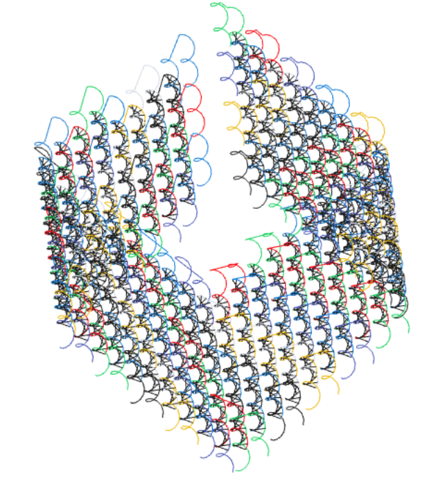
A somewhat unrealistic cubic shape specified in codenano by the previous code.
Example: DNA origami
Another use of codenano is to design DNA origami. On the next pictures, the scaffold appears in black and the staples are in red and orange.
An origami designed with codenano.
The relaxed form of the previous design. It is not too different from the previous picture and helices are not intersecting. Thus the design seems to be feasible according to codenano.
When designing origami, the user can download the sequences of the DNA staples needed to create the structure in a test tube.
How codenano relaxes a design
After specifying a design using code, one can relax the design by clicking the relax button in codenano. This section gives an overview of that relaxation procedure.
Modelling DNA Geometry with springs
Codenano models some of the properties of DNA in a coarse-grained way to help the user asses the feasibility of a design. A strand of DNA can be seen as a succession of bases, and when a pair of strands bind they arrange themselves into the shape of a right-handed double helix. In codenano the sequence of covalent bonds between two successive bases is modeled as a single, relatively strong, linear spring. Two bases facing each other on the double helix form a base pair, also modeled as a strong linear spring. Two successive base pairs stack together with an angle that gives the characteristic double helical shape of DNA, that angle is modeled as a weak torsional spring.
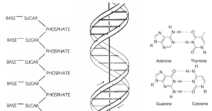
Schematic representation of the DNA molecule. The left and the middle panel were extracted from
the paper by Watson and Crick in Cold Spring Harbor symposia on quantitative biology (Vol. 18, pp. 123-131), Cold Spring Harbor Laboratory Press.
The codenano model for design relaxation
The codenano model consists of a multigraph, which means that we have a set of vertices, and a number of subsets of vertices (muliedges) called the elements.
We model each nucleotide base as a vertex. A vertex has an associated point in 3D space.
There are three kinds of elements:
-
A covalent link. In our model, a single covalent link models the sequence of covalent bonds along the DNA backbone that join two nucleotides. This element is a set of two vertices, since it connects exactly two nucleotides (and hence is an undirected edge rather than a strict multiedge). An example is shown in red below. In the relaxation procedure, covalent links act as a linear spring to hold nucleotide vertices at a defined distance apart.

A covalent link is shown in red. During the relax procedure, the force exerted by the linear spring between A and B is a function of the length AB. -
A hydrogen bond link between paired nucleotide vertices that models hydrogen bonding as an undirected edge. Two hydrogen bond links are shown in red in the image below. In the relaxation procedure, a pair of nucleotides are brought together, but not as closely as a covalent link.
-
A stack, that models the stack between two pairs of nucleotide bases on a pair of DNA strands with no nicks permitted in the stack. Modeled as a multiedge, as a stack involves four nucleotides, where each of the 4 bases are labeled so that codenano knows which of the bases are involved in which of the strands and base pairs. In the relaxation procedure, the stack induces a torsion between the two consecutive base pairs, shown using the angle α in the image below.

Stacks are represented by torsion springs. The force exerted by the stack involving A, C, B and D is a function of the angle $\alpha$.
In summary, the vertices of the multigraph model DNA nucleotides, and each vertex is involved in one to five elements: one or two covalent bonds, up to one hydrogen bond and up to two stacks. The relaxation procedure (relax button) attempts to minimize the force applied to all vertices. See Future work below for features that are not in the current version of codenano.
Finite element method
The vertices define a shape in 3D. To compute a relaxed form of the shape, we use a method called the finite element method.
An element applies a force on each of the nucleotides that it involves. That force is in turn a function of the positions of the nucleotides involved in the element. For example, a spring between two nucleotides $A$ and $B$ applies a force $k\cdot (\|\overrightarrow{AB}\|2 - l_0) \frac{\overrightarrow{AB}}{\|\overrightarrow{AB}\|_2} $ on $A$, where $k$ is the _spring constant of the spring and $l_0$ is the characteristic length of the spring.
There is therefore a vector of forces associated to each set of positions of nucleotides. A relaxed shape is a set of 3D positions where those forces have small norms.
Newton's method for an underconstrained problem
A relaxed shape is a configuration in which all the vertices of the system have a very small force applied on them. As described above, the vector of forces is a function of our shape and we can say that a shape is relaxed if it is a root of this function (all forces are zero). To find an approximation of this root we use Newton's root-finding method.
Let $S_n$ be our shape at iteration $n$, and let $|S_n|$ be the number of vertices in $S_n$. To compute iteration $n+1$, we need to compute the vector of forces $F$, where $F$ is of length $3\cdot |S_n|$, and entries $F[3i]$, $F[3i + 1]$ and $F[3i + 2]$ are respectively the $x$, $y$ and $z$ components of the force applied on vertex $i$. We also need to compute the Jacobian matrix $J$ where $J[i,j]$ is the partial derivative of $F[i]$ with respect to the coordinate $j$. Once $F$ and $J$ have been computed we can compute the next iteration $S_{n+1}$
$S_{n+1} = S_n + \Delta$
Here $\Delta$ is a solution of the linear system,
$J\Delta = -F$
This leaves us with two more challenges: computing $J$ and solving the linear system above.
Implementation
Automatic differentiation
Computing the vector $F$ is easy. At each iteration, all the vector's components are set to 0, and we iterate over all of the elements of our system. Each element updates the components corresponding to the points that it involves. To do so, an element has a method associated to each of its points that computes the force applied to this point as a function of the positions of all the points involved in the element. An element involving $n$ points is therefore associated to $3n$ functions of $3n$ variables (one variable for each of the 3 coordinates of each point).
Computing the matrix $J$ is similar. At each iteration, all the components are set to 0 and each element updates the coordinates that it must update. But now, an element involving $n$ points must have $(3n)^2$ methods that compute the partial derivatives. In the case of the torsion spring, $n=4$ so that mean that $(3\cdot 4)^2 = 144$ partial derivatives have to be computed, and writing a procedure for each would be tedious, so we must find a clever way to do it. Also, to make it easy to extend codenano in the future, we want an approach that makes it easy to implement new elements without having to code up large numbers of complicated and tedious derivatives.
We decided to implement a method do perform automatic differentiation. To do so, we designed a recursive data structure to represent arithmetic expression.
enum FormalEnum<F: Float> {
    Var(usize),
    Const(F),
    Mult(Formal<F>, Formal<F>),
    Add(Formal<F>, Formal<F>),
    Neg(Formal<F>),
    Div(Formal<F>, Formal<F>),
    Cos(Formal<F>),
    Sin(Formal<F>),
    //[...]
}
#[derive(Debug)]
pub struct Formal<F: Float>(Rc<FormalEnum<F>>);
The Chain rule turns the computation of derivatives into a recursive procedure. This is all we need to implement the method Formal::derive.
impl<F> Formal<F> {
    pub fn derivative(&self, n: usize) -> Self {
        let Formal(ref me) = *self;
        match **me {
            FormalEnum::Var(m) if n == m => Formal(Rc::new(FormalEnum::Const(F::one()))),
            FormalEnum::Var(_) | FormalEnum::Const(_) => {
                Formal(Rc::new(FormalEnum::Const(F::zero())))
                },
            FormalEnum::Mult(ref a, ref b) => {
                a.derivative(n) * b.clone() + b.derivative(n) * a.clone()
            },
            FormalEnum::Add(ref a, ref b) => a.derivative(n) + b.derivative(n),
            FormalEnum::Cos(ref m) => m.derivative(n) * -m.sin(),
            FormalEnum::Sin(ref m) => m.derivative(n) * m.cos(),
            }
            //[...]
        }
    }
}
However, for performances reasons, we don't want those recursive data structures to be used during the actual computation. Instead these types are used in procedural macros to generate the code that defines the elements.
For example, the code below shows how to define a spring. Note that we only have to explicitly express the forces and not the derivatives which are automatically computed.
 pub struct _Spring{}
impl<F: Float> AutoImplementable<F> for _Spring {
   fn struct_name() -> String {
       String::from("Spring")
   }
   fn elt_list() -> Vec<String> {
       vec![String::from("a"), String::from("b")]
   }
   fn cst_list() -> Vec<String> {
       vec![String::from("l"), String::from("k")]
   }
   fn formal_map() -> HashMap<String, FormalVector<F>> {
   //Create a `Formal` for each element coordiate and each constants
       let point_a = FormalPoint {
           x: Formal::new_var(0),
           y: Formal::new_var(1),
           z: Formal::new_var(2)
       };
       let point_b = FormalPoint {
           x: Formal::new_var(3),
           y: Formal::new_var(4),
           z: Formal::new_var(5)
       };
       let cst_l = Formal::new_var(6);
       let cst_k = Formal::new_var(7);
       // The force applied on point a is k(|ab| - l) * ab/|ab|
       let ab = point_b - point_a;
       let force_a: FormalVector<F> = (ab.clone().norm() - cst_l.clone())
                                            * ab.clone()/ab.clone().norm()
                                            * cst_k.clone();
       // The force applied on point b is k(|ba| - l) * ba/|ba|
       let force_b = (ab.clone().norm() - cst_l.clone())
                     * ab.clone()/ab.clone().norm() * cst_k.clone()
                     * Formal::new_cst(F::one().neg());
       let mut ret = HashMap::new();
       ret.insert(String::from("a"), force_a);
       ret.insert(String::from("b"), force_b);
       ret
   }
}
// Once the trait is implemented, we can write a procedural macro
\#[proc_macro]
pub fn auto_impl_spring(_item: TokenStream) -> TokenStream {
   macro_def::<f32, _Spring>()
}
Solving sparse underconstrained linear systems
The Jacobian matrix $J$ defines a linear system of equations that we must solve at each step of Newton's method. If $J$ is invertible then the associated linear system has one unique solution. This might not be the case in our situation because multiple distinct configurations of the nucleotides might satisfy the physical constraints. Moreover, the time complexity of solving general linear systems grows quickly with their size. But our system has one big advantage: Since all of the constraints that we consider are local, the Jacobian matrix is sparse. There is an algorithm that can take advantage of the sparsity of a matrix to solve quickly the associated linear system. The LSQR algorithm has both the advantages of being able to solve underconstrained linear systems, and to take advantage of sparsity. There is a C implementation of this algorithm. We took that implementation and rewrote it in Rust.
A crate to use finite element systems in Rust.
The Finite element system solver that we wrote for codenano is available as a crate. This crate comes with another to define new types of finite elements.
End result: architecture, in-browser API
The user can write code on the client. The Rust code is sent to the server, compiled and run by Cargo on the server, producing a datastructure containing tentative positions of the helices and nucleotides. Then, the client web browser receives the WASM version of the Finite Elements solver described above, as well as a WebGL visualiser, and runs the solver, displaying the current result in the WebGL canvas at each iteration.
These tools allows user to create their designs using a Rust API. The user can specify the positions and orientations of DNA helices, draw strands on these helices and connect them with jumps, all in their web browser.
Future work
Codenano could still benefit from many features. As indicated above, there are many aspects of DNA that are not modeled by codenano, and in particular not modeled in the relaxation procedure. codenano is written in such a way that some of these features could be included in future versions while maintaining efficient (fast, low memory) execution via sparse matrix calculations.
- helix rigidity, alignment of consecutive stacks;
- blunt end stacking, stacks with a nick;
- mismatch loops, bulge loops, end of helix loops;
- steric hindrance, volume exclusion, charge repulsion of DNA strands.
Credits and Funding
Codenano was developed by Nicolas Levy and Pierre-Étienne Meunier, while working in the TAPDANCE research group of Damien Woods. Valuable feedback was provided by Coline Petit-Jean and Nicolas Schabanel.
This research was supported by European Research Council (ERC) under the European Union's Horizon 2020 research and innovation programme (grant agreement No 772766, Active-DNA project to Woods), and Science Foundation Ireland (SFI) under Grant number 18/ERCS/5746 to Woods.