Tristan and I have a new paper on the Collatz process, to appear at the 14th International Conference on Reachability Problems.

The Collatz process is simple to describe: Pick a number. If your number is even then divide it by two, if it is odd then multiply by 3 and add 1. And repeat! For example, if we start with 10, which is even, we then get 5. Which is odd, so we get 16. Then 8 then 4 then 2 then 1 then 4 then 2 then 1 ... we are in a loop! The Collatz conjecture says that no matter which natural number \( 1,2,3,\ldots \) you start with you will eventually end at 1. It has been shown to hold for all natural numbers up to \(10^{20}\) (roughly) by computer simulation, but a proof that it holds for any natural number remains elusive, and the problem seems notoriously hard to solve.

Running Collatz by hand kinda feels like the step-by-step process of running an algorithm, and it turns out that deep connections with the theory of algorithms lie just around the corner. John Conway has shown that if we generalise Collatz so that instead of asking whether a number \(x\) is odd or even, aka taking \(x \mod 2\), we take a somewhat larger mod than 2, and allow for 1-variable affine equations with rational coefficients (of the form \(ax+b\)), then we can express any algorithm we want as a Collatz-like process! Such a universal generalised Collatz system works by simulating a counter machine, which in turn simulates Turing machine, and thus any algorithm. Since generalised Collatz systems run algorithms, this means that there is a whole spectrum of algorithmic behaviours buried inside these deceptively simple-looking systems. In that light, it seems natural (to us anyway!) to ask: what kind of computational behaviours are buried 'under the hood' in the Collatz process itself? Maybe the reason Collatz is hard to understand is that it embeds some crazy algorithms that are doing tricky computations. Our goal is to understand Collatz a bit better by thinking in this computational way.

A Collatz machine

Our paper applies a kind of microscope, as Tristan calls it, to look deeply into what happens to numbers that get churned through the Collatz "sausage machine". We define a model of computation that we call the Collatz Quasi Cellular Automaton, or CQCA—it just rolls off the tongue, just like xkcd. The automaton runs Collatz iterations and (essentially) does nothing else, one can think of this as a kind of 'Collatz machine'. You give it a number as input, written in base 2 or base 3, then watch the machine go, and it computes iterations of the Collatz map.

If you want to give the input in base 2 you write it horizontally, with the least significant bit on the right:

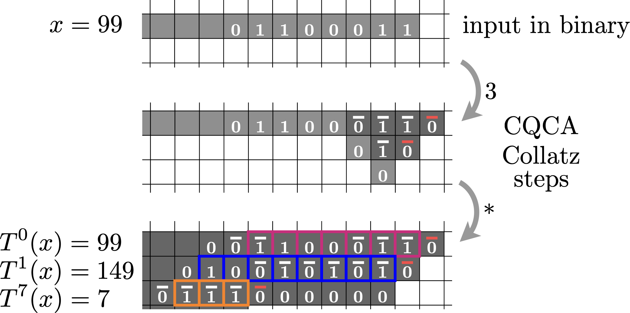
After some time we see the first Collatz iteration (\(T^1(99)=149\), in blue), and after some more time we see the seventh iteration (\(T^7(99)\), in orange). On each line we see an odd iteration of Collatz, meaning an iteration that results in an odd number. The remaining even iterates are also there, one simply needs to appropriately interpret the leading 0s. For example, even iterates \(T^2\) to \(T^6\) appear on the same row as \(T^7\), each using one less leading zero.

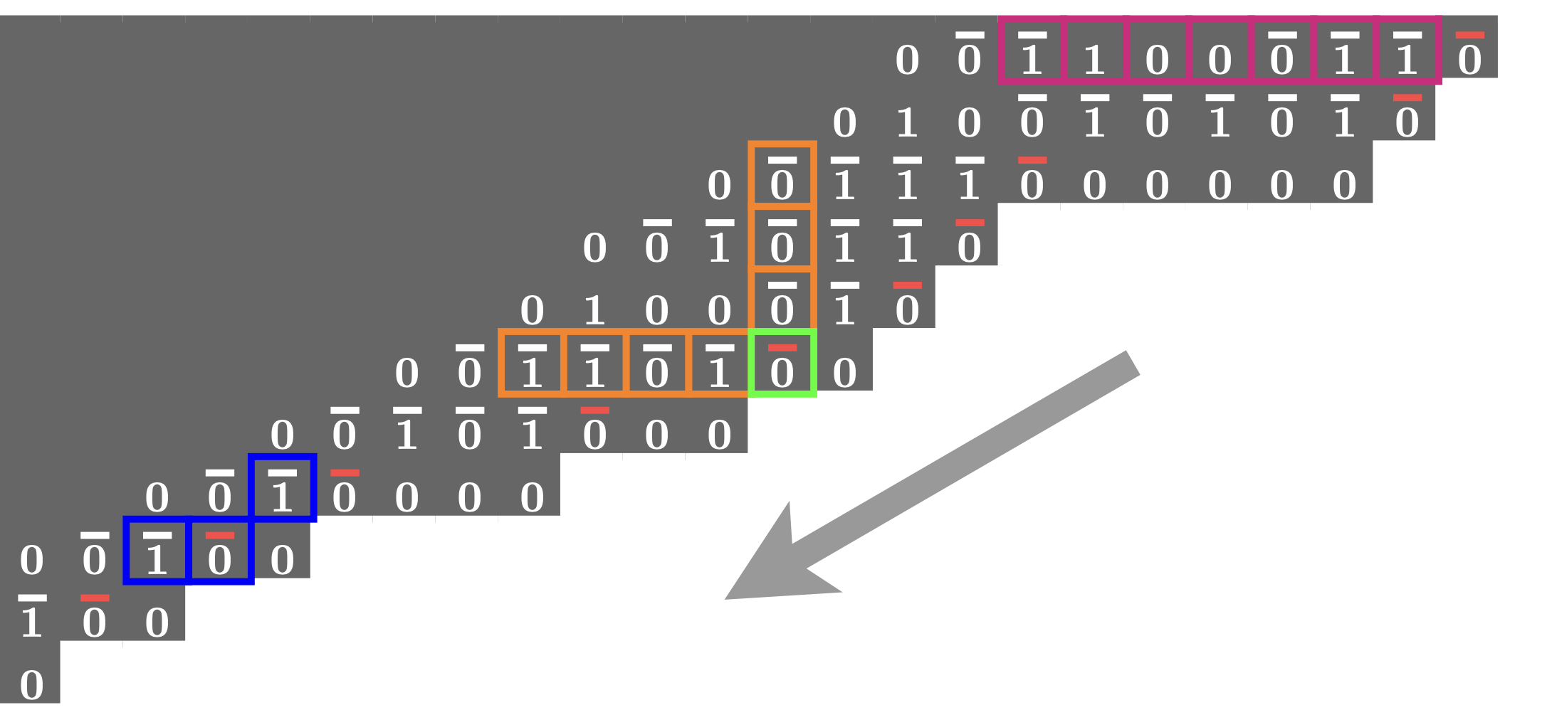
If we let it run on, we would see a full (infinite) execution of Collatz, as the following picture shows. In blue, we see the number 1 highlighted (in two different places), and then the system loops forever down and to the left.

If you want to give the input in base 3 you would write¹ it vertically on a column.

Base 3-to-2 conversion in Collatz

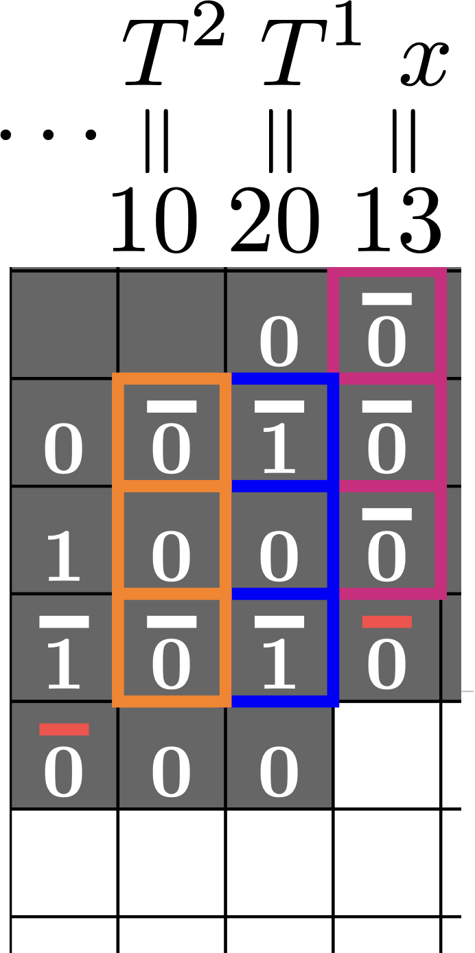
Here's the crazy thing, if you give an input \(x\) in base 3, and wait a while, then you will see your same input get transformed into base 2. In other words, while it is running Collatz the CQCA is converting from base 3 to 2.

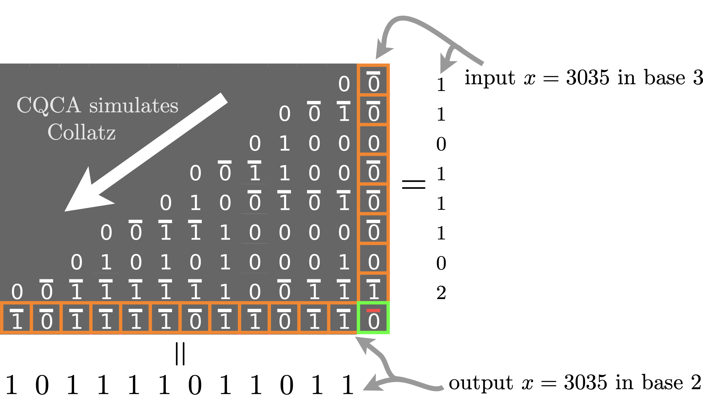
It turns out that almost every cell in the diagram has what we call the base conversion property: the column above the cell contains a number written in base 3, and the horizontal row to the left of the cell has that same number written in base 2. The green cell above has that property, but so does every other cell in the picture! We also get that the CQCA diagrams are filled with parity-checking bits: each 0/1 bit in the center of a cell is exactly the parity (0 or 1) of the number of 1s (we include carries) in a neighbouring vertical column of cells: for example, the parity of the orange column above (it contains 7 ones, so the parity is 1) is in the cell to the left of the green cell. In general, the parity of the entire vertical column is found in the cell immediatly below and to the left of that column. All this happens while the CQCA is executing Collatz, and doing so rather efficiently, hence base conversion, and parity checking, seem intricately woven into the fabric of the Collatz process.

This behaviour would perhaps be unsurprising if the CQCA was a complicated beast (like your computer) that computed Collatz iterations while, say, also running a SAT solver, analysing some data and drawing stuff on a screen. But its not, all it does is run Collatz. To get a better handle on what this means lets pick up the hammer of computational computational complexity theory and whack a few nails.

Computational complexity of the Collatz process

In roughly \(O(n)\) steps the CQCA runs a base conversion algorithm, but we'd like to classify more generally the power of this Collatz machine. So how much computation is really happening here? In the long term, the answer is "we don't know", mainly because the Collatz problem remains unsolved. However, it turns out that we can say something in the short term. In the paper we choose to look at a what happens in a kind of "bounding box" of distance \(O(n)\) from the \(n\)-trit input.² What we really want to know is how difficult is it to predict these bits/trits knowing just the input.

The maximum difficulty, or complexity, we would have here if instead of the CQCA we had (say) an arbitrary cellular automaton, or an arbitrary Turing Machine, would be something called P-completeness. This technical-sounding term means that we can compute these bits on a polynomial (in \(n\)) time Turing Machine, but doing so would be as hard as any problem in P. In this \(n\)-bounded setting, we think of P-completeness as being "pretty damn hard"; there are unlikely to be fancy shortcuts, closed form formulae, or other tricks to make the simulation any easier. But we don't have an arbitrary algorithm (we believe!), we have Collatz, or more accurately, we have the CQCA.

The base conversion result gives us, almost for free, that computing about half the bits/trits from our \(n\)-trit input lies in NC¹, but outside of AC⁰. In lay-person terms this means that these bits can be computed very quickly and independently (in parallel) from each other, a parallel computer can compute them in \( O(\log n) \) time. But can not much better than that.

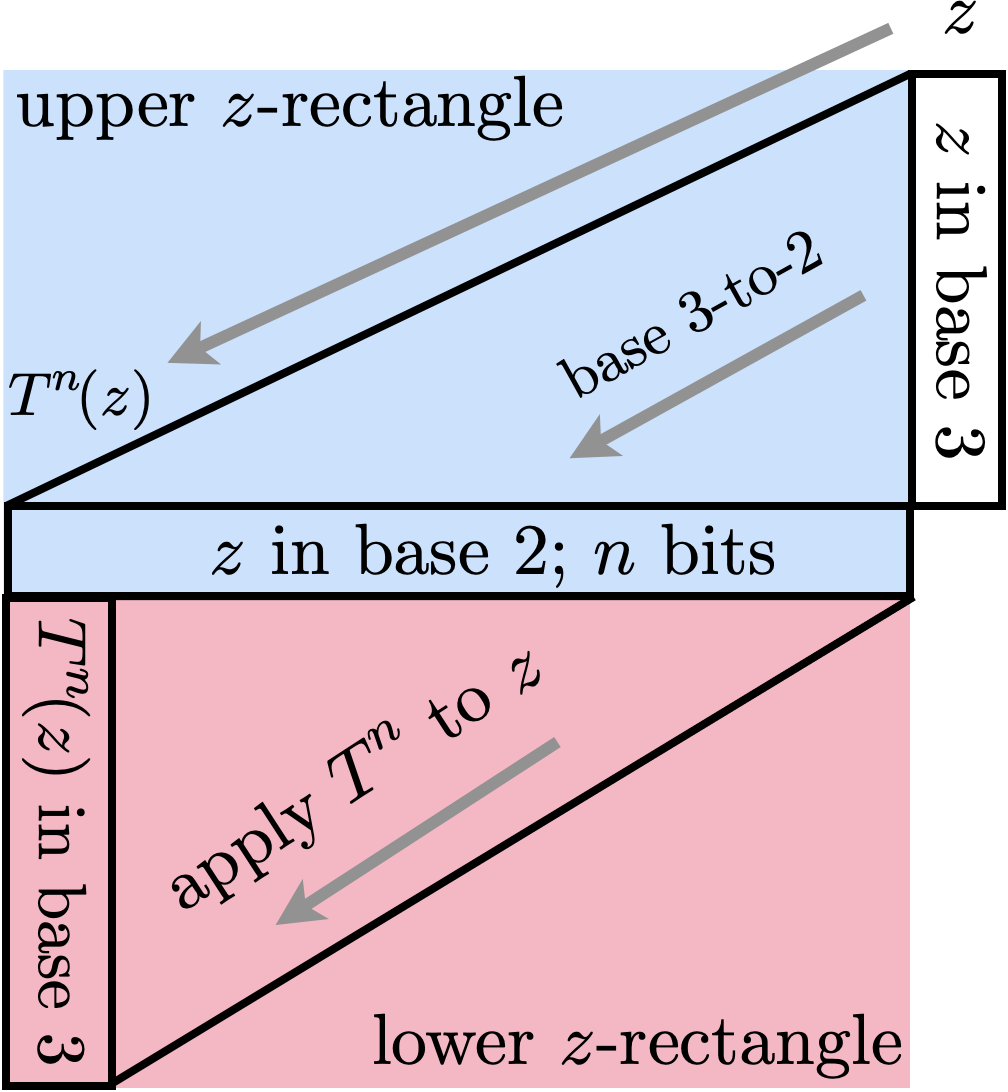
But what about the other half of the bits/trits? Beyond saying that they are in P, we just don't know ... yet. In some sense, predicting these bits seems at least as hard as predicting all the bits, since it encodes \(n\) steps of Collatz, although in a weird base-changing way shown in the bottom half of the following image.

I've intentionally left out a lot of details and extra results here, but you can read the paper, or play with Tristan's simulator, to learn more.

These pictures tell us there is some underlying structure to Collatz iterations. The next big question is whether this kind of structure could be useful in getting a better understanding of its long-term dynamics.

¹Technical caveat: Base 3 typically uses the symbols 0,1,2, but here we are using a version of base 3 where there are two ways to write the digit 1, either as \(1\) or as \(\overline{0} \). See our paper for the reason why. We call it base 3'.

² A trit is like a bit, but there's three of them.